Super Agents of AI

Competition Mechanics

• Main concepts:
  • Data
  • Model
  • Submission
  • Evaluation
  • Leaderboard
• Competition platforms
• Reasons for participating

Real Life VS Competition

Real Word ML Pipeline

It’s a complicated process included:

• Understanding of business problem
• Problem formalization
• Data collecting
• Data preprocessing
• Modelling
• Way to evaluate model in real life
• Way to deploy model

Things We Need to Care about

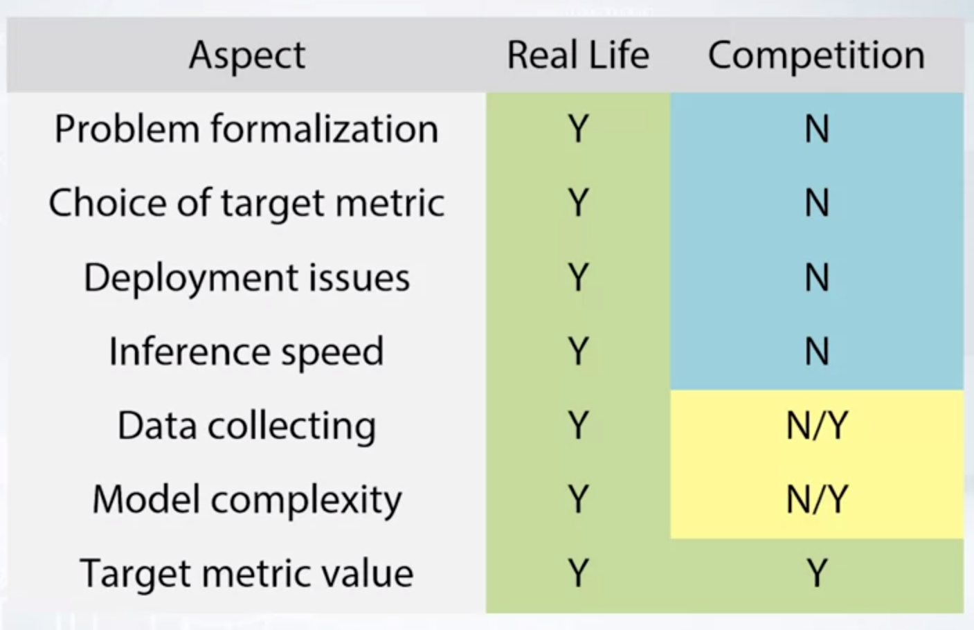
Real-world problems are quite complicated. Competition are a great way to learn, but they don’t address the questions of formalization, deployment and testing.

Recap of Main ML Algorithms

Families of ML Algorithms

• Linear
  • Logistic Regression
  • Support Vector Machine
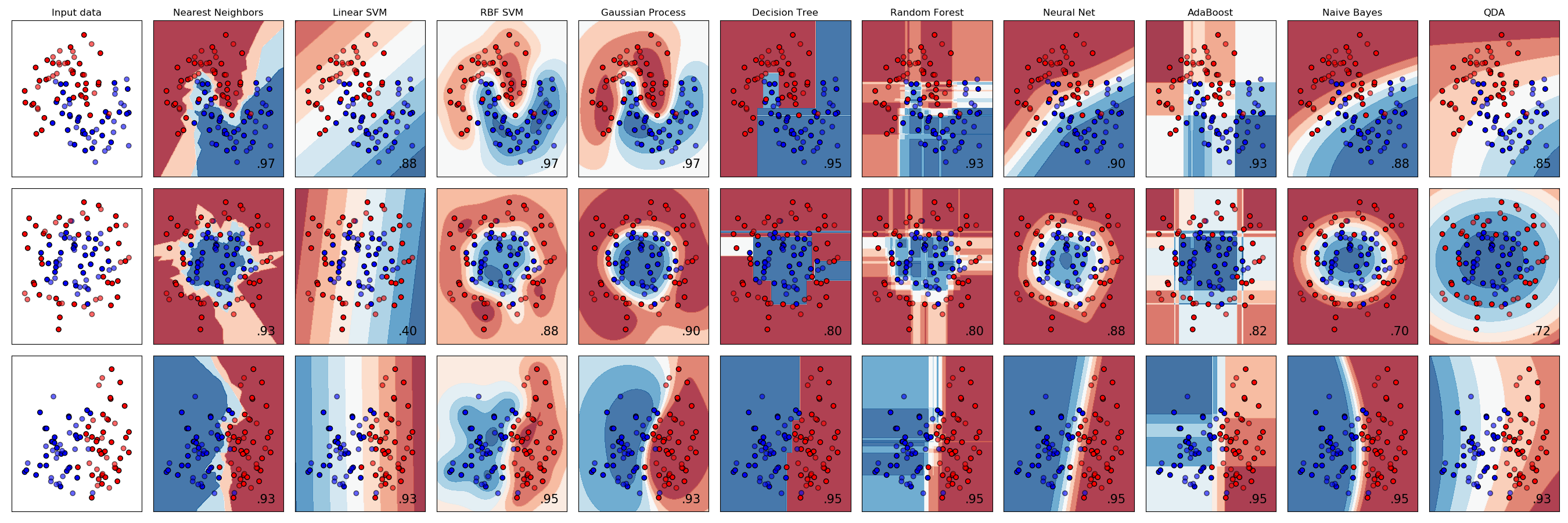
  • Linear models split space into 2 subspaces
• Tree-based
  • Decision Tree, Random Forest, GBDT
  • Scikit-learn, XGBoost, LightGBM
  • Tree-based methods splits space into boxes
  • ExtraTrees classifier always tests random splits over fraction of features (in contrast to RandomForest, which tests all possible splits over fraction of features)
• KNN
  • KNN methods heavy rely on hot measure points “closeness”

• Neural Network

  • Feed-forward NNs produce smooth non-linear decision boundary

• Trees in RandomForest can be constructed in parallel (that is how RandomForest from sklearn makes use of all your cores). Since each tree is independent from other trees

• In GBDT each new tree is built to improve the previous trees. The idea of boosting is to correct errors of previously learned models

The most powerful methods are Gradient Boosted Decision Trees and Neural Networks. But you shouldn’t underestimate the others

No Free Lunch Theorem

Here is no method which outperforms all others for all tasks

There is no “silver bullet” algorithm

Classification Results of Different Methods

Feature Preprocessing and Generation with Respect to models

• Feature preprocessing is often necessary
• Feature generation is powerful technique
• Preprocessing and generation pipelines depend on a model type

Preprocessing: Scaling

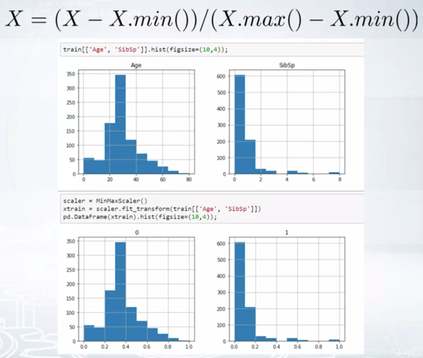
• To [0,1]:

  • Sklearn.preprocessing.MinMaxScaler

  $$ X = \frac{X - X.min()}{X.max() - X.min()} $$

• To mean=0, std=1:

  • Sklearn.preprocessing.StandardScaler:
    

  $$ X = \frac{X - X.mean()}{X.std()} $$

Preprocessing: Outliers

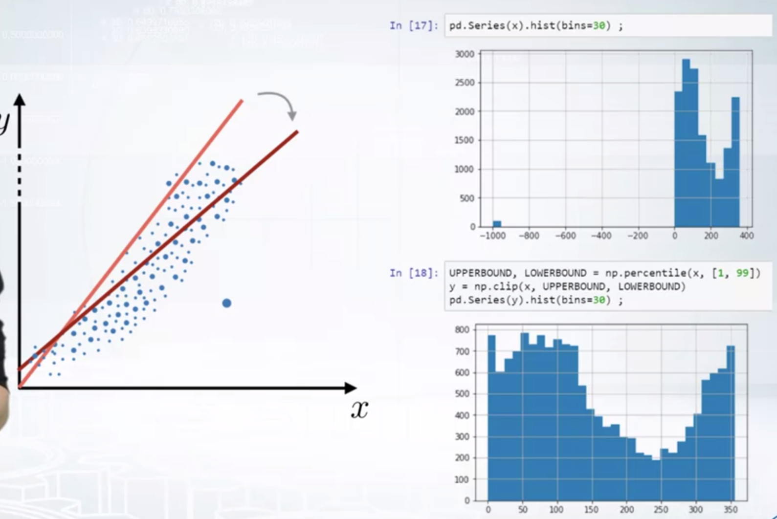
Clipping the values using winsorization method:

• Apply rank transform to the features. Yes, because after applying rank distance between all adjacent objects in a sorted array is 1, outliers now will be very close to other samples.
• Apply np.log1p(x) transform to the data. This transformation is non-linear and will move outliers relatively closer to other samples.
• Apply np.sqrt(x) transform to the data. This transformation is non-linear and will move outliers relatively closer to other samples.
• Winsorization. The main purpose of winsorization is to remove outliers by clipping feature’s values.

Preprocessing: Rank

It sets spaces between sorted values to be equal.

• rank([-100, 0, 1e5]) == [0,1,2]
• rank([1000, 1, 10]) == [2, 0 , 1]
• scipy.stats.rankdata

Other Preprocessing Methods

• Log transform: np.log(1+x)
• Raising to the power < 1: np.sqrt(x + ²⁄₃)
  

Sometimes, it is beneficial to train a model on concatenated data frames produced by different preprocessing methods, or to mix models training differently-preprocessed data. Again, linear models, KNN, and neural networks can benefit hugely from this.

Feature Generation

Ways to proceed:

• Prior knowledge
• EDA

Conclusion

1. Numeric feature preprocessing is different for tree and non-tree models
   1. Tree-based models doesn’t depend on scaling
   2. Non-tree-based models hugely depend on scaling
2. Most often used preprocessings are:
   1. MinMaxScalar - to[0,1]
   2. StandardScaler - to mean==0, std==1
   3. Rank - sets spaces between sorted values to be equal
   4. np.log(1+x) and np.sqrt(1+x)
3. Feature generation is powered by:
   1. Prior knowledge
   2. Exploratory data analysis

Categorical and Ordinal Features

Ordinal Features

Values in ordinal features are sorted in some meaningful order.

Label Encoding

Label encoding maps categories to numbers.

• Alphabetical (Sorted)
  • [S, C, Q] - > [2,1,3]
  • sklearn.preprocessing.LabelEncoder
• Order of appearance
  • [S, C, Q] - > [1,2,3]
  • Pandas.factorize

Frequency Encoding

Frequency encoding maps categories to their frequencies.

• [S, C, Q] - > [0.5,0.3,0.2]

encoding = titanic.groupby('Embarked').size()
encoding = encoding/len(titanic)
titanic['enc] = titanic.Embarked.map(encoding)

If the frequencies of the types are equal, we can use the rank to deal with it.

from scipy.stats import rankdata

Categorical Features

One-hot Encoding

• pandas.get_dummies
• sklearn.preprocessing.OneHotEncoder

Conclusion

• Label and Frequency encodings are often used for tree-based models
• One-hot encoding if often used for non-tree-based models
• Interactions of categorical features can help linear models and KNN

Datetime and Coordinates

Date and Time

• Periodicity: Day number in week, month, season, year, second, minute, hour
• Time since
• Difference between dates

Coordinates

• Interesting places from train/test data or additional data
• Centers of clusters
• Aggregated statistics

Handling Missing Values

The choice of method to fill NaN depends on the situation. Usual fillna approaches:

1. -999, -1, etc
2. mean, median
3. Reconstruct value
4. Missing values already can be replaced with something by organizers
5. Binary feature “isnull” can be beneficial

In general, avoid filling NaN before feature generation, since it can decrease usefulness of the features. XGBoost can handle NaN.

Feature Extraction from Texts and Images

Text -> Vector

Text Preprocessing

• Lowercase
• Lemmatization
  • democracy,democratic, and democratization -> democracy
  • Saw -> see or saw (depending on context)
• Stemming
  • democracy,democratic, and democratization -> democr
  • Saw -> s
• Stopwords
  • Articles or preposition
  • Very common words
  • NLTK, Natural Language Toolkit library for python
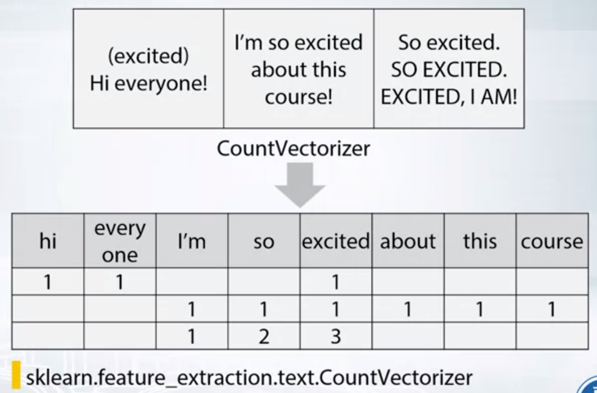
  • Sklearn.feature_extraction.text.CountVectorizer: max_df

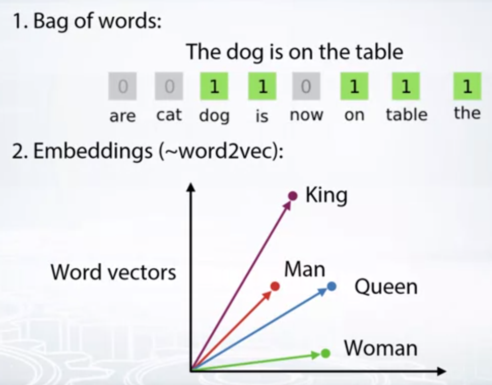
Bag of Words

TF-IDF:

N-Grams:

Pipeline of applying BOW:

1. Preprocessing:
   1. Lowercase, stemming, lemmatization, stopwords
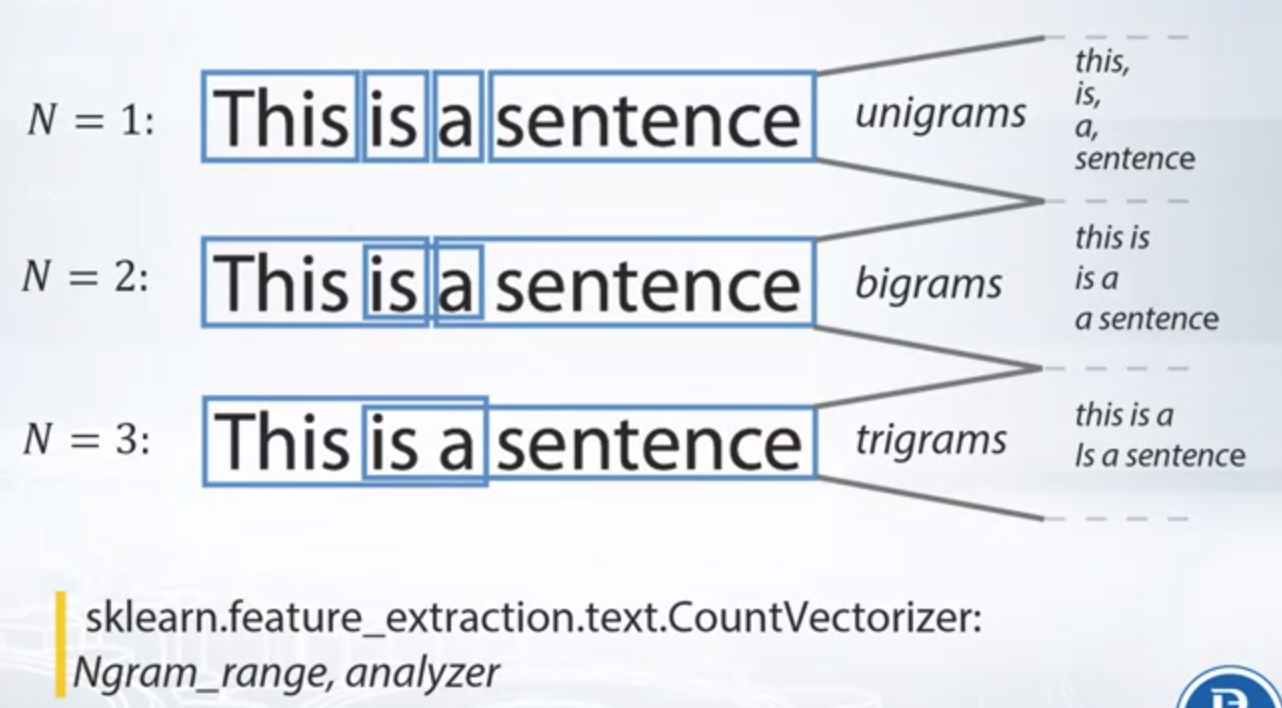
2. N-grams can help to use local context
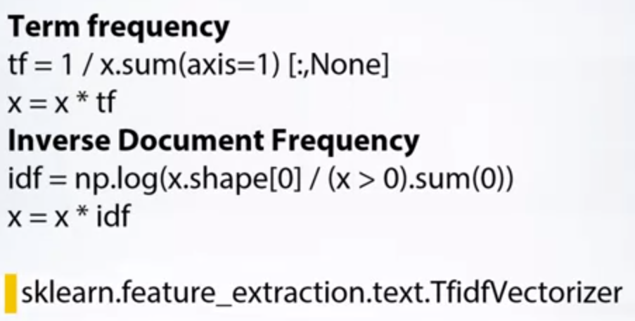
3. Postprocessing: TFiDF

Word2vec

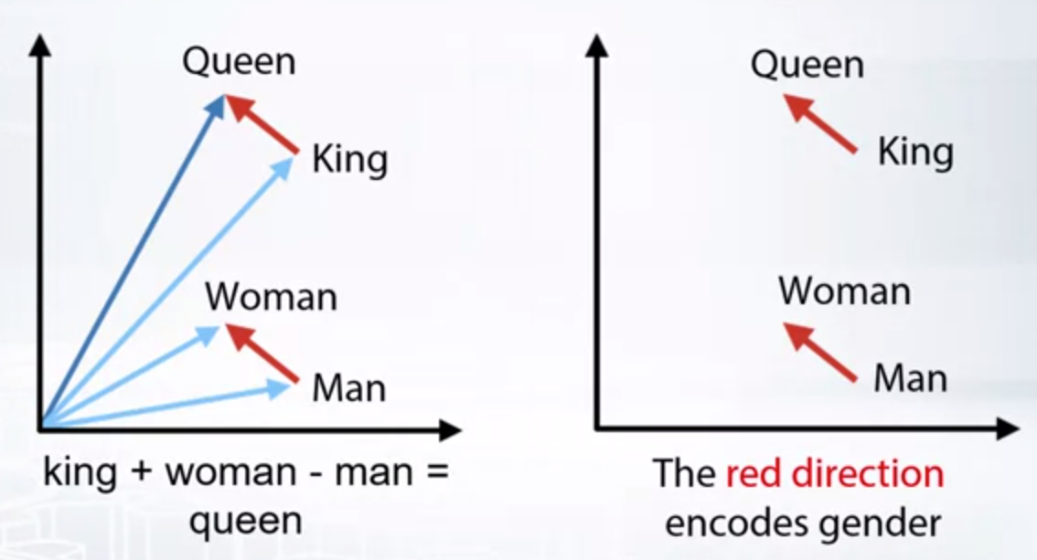
• Words: Word2vec, Glove, FastText, etc
• Sentence: Doc2vec, etc
• There are pre-trained models

BOW and Word2vec Comparison

1. BOW:
   1. Very large vectors
   2. Meaning of each value in vector is known
2. Word2vec
   1. Relatively small vectors
   2. Values in vector can be interpreted only in some cases
   3. The words with similar meaning often have similar embeddings

Image -> Vector

1. Descriptors: Features can be extracted from different layers
2. Train network from scratch: Careful choosing of pre-trained network can help
3. Fine-tuning: Fine-tuning allows to refine pre-trained models

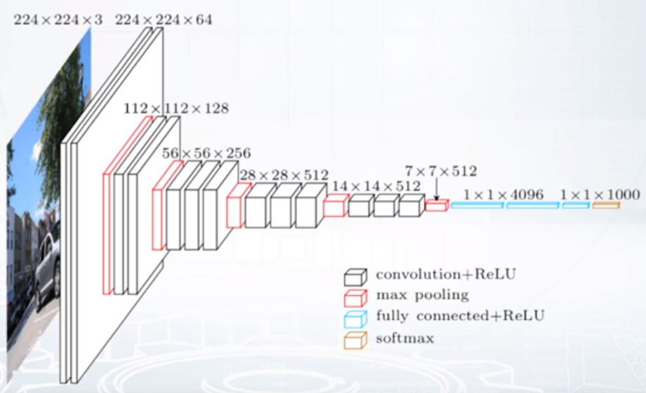
Image Augmentation

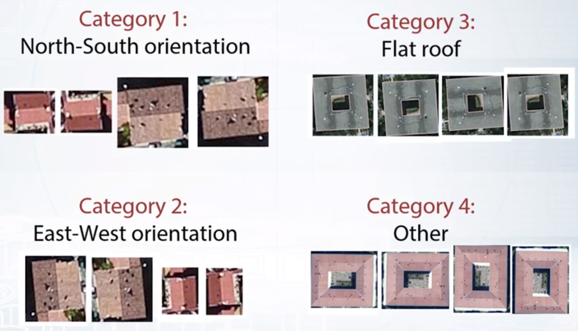
Data augmentation can be used (1) to increase the amount of training data and (2) to average predictions for one augmented sample.

Note: Cover Picture